3 Blasius solution

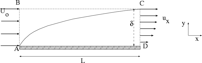
The Blasius problem deals with flow in the boundary layer around a stationary plate. The setup is shown in figure 2. At a large distance the fluid has a uniform velocity U. It interacts with a plate whose edge is at x = 0 and which extends to the right from there. As before, we need to think about the physical situation that we expect to develop before tackling the mathematics. Thus, at x = 0 fluid right at the surface of the plate must be brought to rest (u_x = 0). As before, the effect of the presence of the plate propagates outwards into the fluid, ie the boundary layer becomes broader. However at the same time the fluid is flowing downstream along the plate. So instead of the boundary layer getting thicker as time progresses, it instead gets thicker as you move further along the plate.

Figure 2: Boundary layer around a stationary plate - Blasius problem

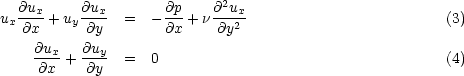
Now fairly obviously the presence of this boundary layer will disrupt the uniform flow of the fluid, and so in the boundary layer the flow will have components u_x and u_y. We will assume that the growth of the boundary layer is quite slow, i.e. its thickness is small compared to x at any point x down the plate. In this case u_y < u_x, and the Navier-Stokes equations simplify to

In fact it is best to write u_x and u_y in terms of a stream function

(5)

Thus, if we can solve equation 5 to find f(), we can find the flow throughout the boundary layer. In particular, the friction coefficient