I.5 Temporal discretisation
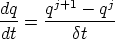
This problem is a parabolic one : we have a set of values representing the solution at one time
step, and we will solve the equations by computing successive timesteps. This timestepping
represents a discretisation of time as well as space into M timesteps qj. The time derivative
can thus be expressed as
 We can insert this into (I.5). This raises the question : at what timestep are the values on the
r.h.s. evaluated? If we assume they are taken as the values at timestep j, then we have an
explicit scheme. If we use the values at timestep j + 1 then we have an implicit
scheme.
We can insert this into (I.5). This raises the question : at what timestep are the values on the
r.h.s. evaluated? If we assume they are taken as the values at timestep j, then we have an
explicit scheme. If we use the values at timestep j + 1 then we have an implicit
scheme.
For an explicit scheme we can write this as
 We can write this in terms of 2 factors
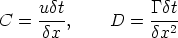 C is the Courant number for the problem, and is a significant parameter in determining the
stability of the scheme. D is a similar parameter relating to the diffusion. Writing this out as
an algorithm :
C is the Courant number for the problem, and is a significant parameter in determining the
stability of the scheme. D is a similar parameter relating to the diffusion. Writing this out as
an algorithm :
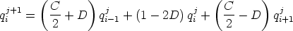 | (I.6) |
This is a rule for advancing the values of q through one timestep, which could be written into a
spreadsheet.
In the case of the implicit scheme we would write the scheme in terms of a vector of
unknown values (qij + 1), as a matrix equation :
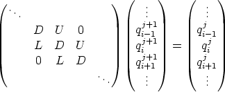 where D, U and L are constant values related to C and D. Inverting this matrix provides the
solution without the stability problems mentioned above (although the Courant number is still
worth calculating if there are problems).
where D, U and L are constant values related to C and D. Inverting this matrix provides the
solution without the stability problems mentioned above (although the Courant number is still
worth calculating if there are problems).