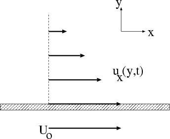
2 Impulsively started plate
We will start by looking at a simple laminar boundary layer, formed when a plate starts moving in a stationary
fluid. This is referred to as an impulsively moving plate. Initially the plate and the fluid around it are
stationary. At time t = 0 the plate begins to move sideways (see figure 1) with speed U0. This will have an
effect on the fluid immediately surrounding the plate, which will start moving with the same speed. This will
then influence fluid a bit further out, which will begin to move (a bit slower). This in turn will
influence the next layer of fluid, which will start to move. The important point to notice is that it
takes time for each layer of fluid to influence the next one out. Hence we expect a moving layer
of fluid to develop around the plate - the boundary layer - which will grow outwards as time
progresses.
If this is the case - i.e. there is no flow in the y direction, and no variation in the flow in the x direction (the
plate is assumed to be infinitely long).
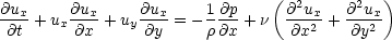
The momentum equation in 2d cartesian coordinates is
 For this case we would expect to get a solution for this problem of the form ux(y, t) - i.e. there is no flow in the
y direction, and no variation in the flow in the x direction (the plate is assumed to be infinitely long). This
implies
For this case we would expect to get a solution for this problem of the form ux(y, t) - i.e. there is no flow in the
y direction, and no variation in the flow in the x direction (the plate is assumed to be infinitely long). This
implies
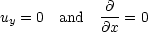 and so the momentum equation reduces to
 | (1) |
However this is still a partial differential equation (P.D.E). To solve it we need to reduce it to an ordinary
differential equation (O.D.E). We can do this via a technique known as Combination of Variables. Let us
assume that ux is a function of a single variable  :
:
 where
where
 is a dimensionless variable. (Note that this is another example of the use of dimensional analysis in problem
solving - y, t and
is a dimensionless variable. (Note that this is another example of the use of dimensional analysis in problem
solving - y, t and  are the only dimensional parameters in the problem, and so we can see that the solution
must depend on some dimensionless combination of these parameters). Using the chain rule of differentiation
we can show that and
are the only dimensional parameters in the problem, and so we can see that the solution
must depend on some dimensionless combination of these parameters). Using the chain rule of differentiation
we can show that and
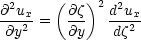 so equation 1 becomes
 | (2) |
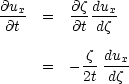
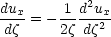
- a second order O.D.E, which we can solve. here is a variable which encapsulates both spatial and temporal
variation. Thus as time progresses (t increases) the solution for a given value of corresponds to a physical
point further and further away from the plate (y increases). This corresponds to our notion that the boundary
layer is growing with time.
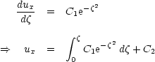
The actual solution of equation 2 is fairly straightforward. If we write
 it becomes
 a 1st order O.D.E, which is separable : i.e. Finally we need to evaluate C1, C2, for which we need to know the boundary conditions.
-
B.C.1
- At y = 0, i.e. at = 0, ux(0) = U0, so
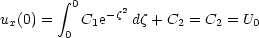 so
so
-
B.C.2
- As y

 , i.e. , ux 0 In this case
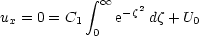 Rearanging this we find
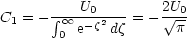
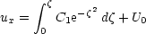
and so
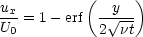
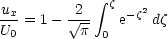 Note that the integral
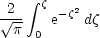 is a mathematical function called the Error Function erf(), with tables of values available. The solution for
this case is thus often written in the form
is a mathematical function called the Error Function erf(), with tables of values available. The solution for
this case is thus often written in the form