I.2 Numerical solutions

Using computers to solve fluid flow problems is basically a 4 stage process.

1. The physical problem has to be modelled. The simplest model would be to describe the flow using the incompressible NSE, but more complex problems may involve models for combustion, heat transfer etc.
2. The resulting equations have to be discretised. Computers cannot take derivatives or work out integrals, all they can do is to manipulate numbers. Thus the modelled pde’s have to be represented by algebraic difference equations involving elementary operations on numbers.
3. These difference equations then have to be solved. This typically involves inverting (finding the inverse of) a very large matrix. Thus the discretisation process gives an equation

   (I.1)

   where M and q are known from our discretisation. If we can find M^-1 numerically, then we can write

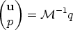   (I.2)

4. This produces, again, a large quantity of numbers. These have to be interpreted - typically displayed graphically (visualisation), analysed to check they are correct, and processed to extract useful information.

Of course, preexisting computer codes already take care of much of this. For instance such codes contain preprogrammed and carefully optimised matrix inversion routines. However, when using such packages there are still choices that need to be made - which of several preprogrammed turbulence models is optimal for a particular case, for example. From the point of view of the informed user, CFD modelling is a 3 stage process :

1. Problem definition. This consists of explaining the problem to the computer, and involves
   • defining the case geometry, and constructing a mesh on which points the solution is to be evaluated
   • selecting appropriate physical models, for instance for turbulence, and providing the correct physical constants such as the fluid viscosity
   • providing initial and boundary conditions for the problem
2. Numerical solution. The next step is to set various numerical parameters in the code and set it to run on the computer. Again, this may involve
   • specifying appropriate differencing schemes to discretise the derivatives, and appropriate solution techniques for solution of the equations.
   • defining tolerances - at what level do we declare the problem to be ‘solved’?
   • actually running the solver on the computer.
3. Postprocessing. This involves displaying the resulting data in a manner to make it easilly understood. Postprocessing techniques may include graphical display on a computer screen, extraction of values at points in the domain, animation of successive timesteps of the solution, or use of virtual reality so that the user can walk into the solution.