Project written by Iestyn Pugh
Introduction
This project had two main aims. These were to increase understanding of computational fluid dynamics (CFD) and to investigate the air flows around the suspension bridge.
CFD allows experiments and analysis of fluid flow to be performed with much less financial and time consuming costs than wind tunnel experiments or physical experiments performed on the body. This means that CFD is a very efficient method of analysing fluid flows.
CFD software packages use computational models to simulate the flow that occurs in reality, in this case the flow around the bridge. A CFD model is made up of the body and the region of fluid around it. This region of fluid is meshed and each cell in the mesh has the flow in and out of it analysed. This enables the CFD software to build up an accurate simulation of the flow around the body. The CFD software package used in this project was Fluent 5.5 and its sister meshing software package Gambit.
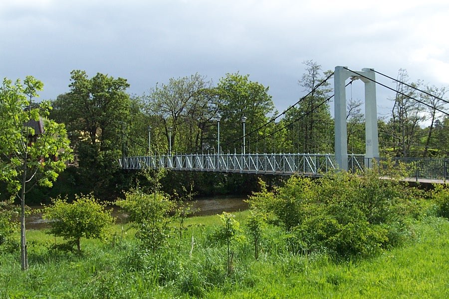
The Trews Weir Suspension Bridge
The bridge that was chosen for the project was the Trews Weir suspension bridge in Exeter. The bridge is shown in the photograph below:
Trews Weir suspension bridge is a traditional pedestrian suspension bridge running over the river Exe. It is located just downstream of Exeter Quay.
To construct a computational model of the bridge the dimensions of the bridge and the physical conditions were required. The bridge was accurately surveyed to obtain the dimensions. The physical conditions that were required for the computational model were the average wind speed, the average temperature and the surface velocity of the river. These were as follows:
Average wind speed = 16 km/h
Average temperature = 10°C
Average river surface velocity = 0.25 m/sCFD Modelling
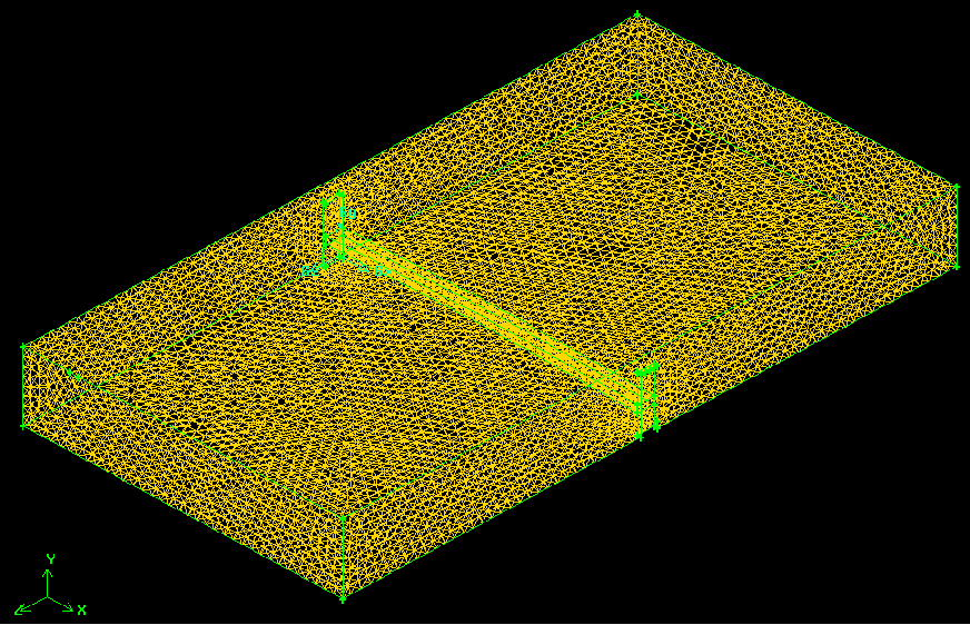
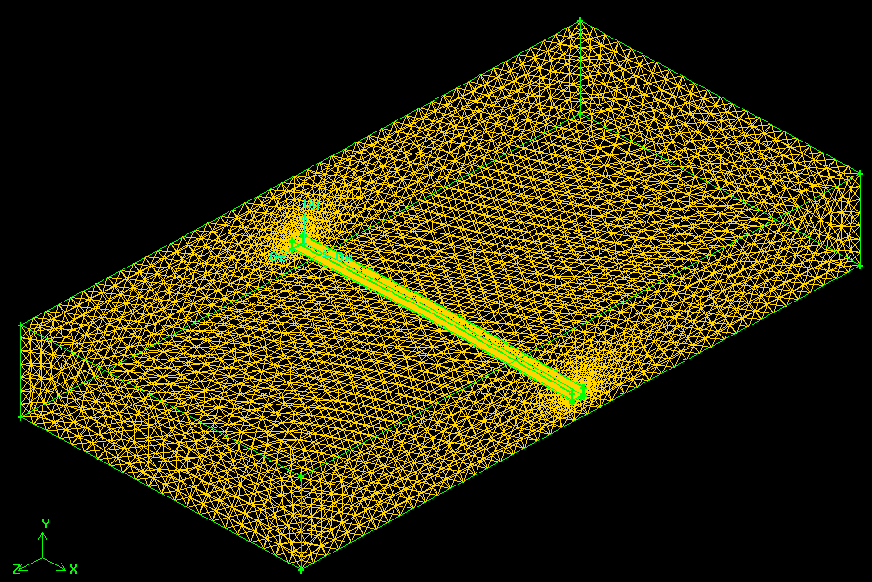
For the CFD solution to be as accurate as possible the computational model should be as close as possible to the actual bridge. In the case of the Trews Weir suspension bridge there is too much detail for Fluent to compute. This means that simplified models have to be created. To cover as much detail as possible two models were created and meshed. These are shown below:
Model A Model B
Flow Patterns
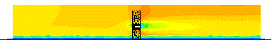
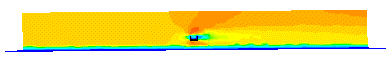
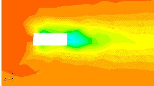
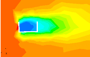
Fluent can produce contour plots of velocity magnitude and total pressure. These enable the flow patterns around the bridge to be visualised. Due to the complexity of the flow, 3-D contour plots do not produce clear flow patterns. To do this a 2-D plane has to be set through the middle of the computational model and the flow patterns can be visualised easily. The diagrams below show the velocity magnitude contour plots of both models:
Model A Model B Both models show similar flow patterns. As the air enters the model (at the left) it flows over the river with the expected boundary layer and as it flows over and under the bridge the flow separates and a turbulent wake is formed. Turbulent wakes are formed by adverse pressure gradients forming on bodies causing boundary layer separation. To see whether this is why the turbulent wakes formed on the computational models total pressure contours were plotted and are shown below:
Model A Model B The diagrams show the formation of an adverse pressure gradient above and below the bridge. As stated previously this pressure gradient causes the boundary layer to separate and a turbulent wake to form behind the bridge.
Experimental Results
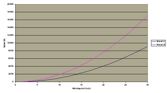
Fluent can also calculate the distributed loads acting on the bridge by the wind. Using this information it is possible to calculate the relationship between wind speed and vertical loading, and the relationship between wind speed and horizontal loading (drag). From this drag relationship it is then possible to calculate the drag coefficients of the two computational models.
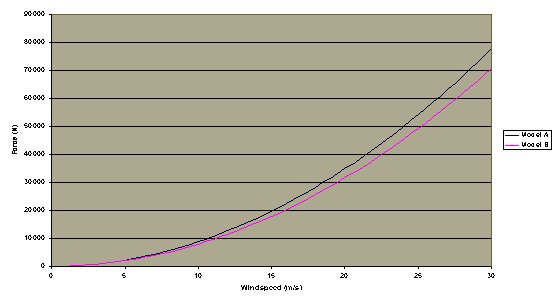
The relationship between wind speed and vertical loading is shown below:
The equations of the lines give the relationship between wind speed and vertical loading:
Model A: Fy = 9.54v2.02 Model B: Fy = 18.6v2.01 The difference in the scale of both models is due to the difference in the geometry of the models. However, the relationship is proven to be a perfect squared relationship.
The relationship between wind speed and horizontal loading (drag) is shown below:
The equations of the lines give the relationship between wind speed and drag force:
Model A: Fy = 94.5v1.97 Model B: Fy = 84.6v1.98 In this case, the relationships are nearly identical. This is due to the similar frontal area of both models. Again, there is a near perfect squared relationship.
Using the drag forces and the following equation it was possible to calculate the drag coefficient of both models:
FDRAG = 0.5*density*CDRAG*area*velocity2
The drag coefficients were calculated and are shown below:
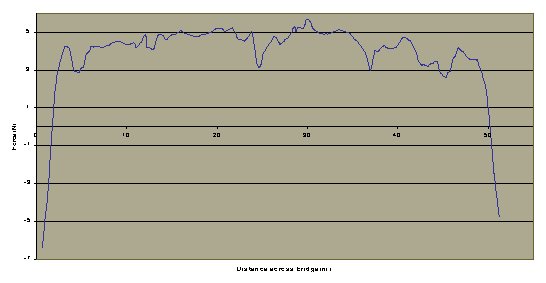
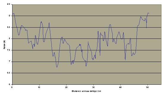
Model A = 1.87 Model B = 2.00 Another function that Fluent is capable of is the calculations of the force distributions acting across the span of the bridge. This experiment was run at the average wind speed of 5 m/s and at 30 m/s which is gale force 11 on the Beaufort scale. The plots of these force distributions at 5 m/s are shown below:
Model A force distribution at 5 m/s
Model B force distribution at 5 m/s
The force distribution plots at 30 m/s for the computational models are the same in shape but the magnitude is much larger.
Conclusions
The aims of the project were to increase understanding of computational fluid dynamics (CFD) and to investigate the air flows around the suspension bridge.
The experiments run in Fluent showed the flow patterns around the bridge and these proved the theory of the adverse pressure gradient forming the turbulent wake behind the bridge. The Fluent experiments also showed that the relationship between wind speed and vertical and horizontal distributed loads is a perfect squared relationship. The drag coefficients for both models were calculated and both models produced similar coefficients. Also force distribution plots were produced showing how the distributed load acts across the span of the bridge.
Understanding of CFD was gained by the use of the two computational models. These showed that CFD isn't the perfect answer to a problem. Approximations and assumptions have to be made for a CFD simulation to be performed. For example, in this case approximations were made with the geometry of the bridge. These approximations and assumptions will obviously effect the solution. However, the advantages of CFD are numeral, these are shown in the introduction section. Therefore, it is possible to say that whilst CFD does have its limitations, there is a very real need for it in both design and understanding of the behaviour of structures in fluid flow.
This web page was written by Iestyn Pugh in May 2002