|
The
effects of parameters on the maximum prediction time possible in short
term forecasting of the sea surface shape
D.R.Edgar, J.M.K.Horwood, R.Thurley and M.R.Belmont.
It has recently been recognised that it is
realistic to make predictions of the detailed of the sea surface shape
typically up to 30 seconds ahead. This offers the prospect of
substantially increasing the operating envelope in a wide range of marine
operations. This article examines, from the point of view of a potential
user of this technology, how the various parameters involved in such so
called Deterministic Sea Wave Prediction System affect the prediction time
and also how prediction time can be traded for precision.
1. Introduction
Statistical forecasting of the sea-state is
of vital importance in marine operations of all kinds. This type of
forecasting may be used as an indicator of conditions in which it may be
impossible to undertake certain types of marine operations. Sea state
critical operations include transfer of materials and personnel between
ships and offshore installations, helicopter operations from ships and
underwater and surface operations managed from ships.
The recent recognition[i],[ii],[iii],[iv],[v]
that it is possible to predict the actual instantaneous shape of the sea
surface, rather than merely its statistics[vi],[vii],
promises to change this situation, offering the prospect of exploiting the
calm periods of a few tens of seconds that exist in some heavy sea
conditions. This could give the opportunity of safely undertaking
operations in sea conditions that would have been previously considered to
render the operation hazardous.
For a large swell sea it is realistic to
expect prediction of the actual shape of the sea surface up to 30 seconds
into the future with surface level prediction errors as low as +
10% of the mean significant wave height2,3. The process of
predicting actual sea surface shape is termed Deterministic Sea-Wave
Prediction, (DSWP). There are a variety of ways of implementing DSWP,
although all of these essentially involve measuring the sea surface in
some manner at a set of locations or over a region remote from the site
(typically 500 m to 1000 m) where prediction is required. The method of
DSWP under discussion here is termed the fixed point method where
measurements are made by sea surface sensors at fixed locations distance
Xpm from the prediction site.
In previous work1,2,3, the basic
principles of DSWP were introduced. The present article explores the
effect of the main parameters affecting DSWP which are likely to be of
importance to potential users of this technique.
A very brief background of the fixed point
method of DSWP theory will be presented followed by a study concerned with
identifying optimum values for the main system variables for a given site,
required accuracy and prediction time.
2. Fixed point method of dswp
For clarity of explanation, the
following discussion is restricted to wave systems arriving at the
prediction site from a single direction. The system can be extended to
multidirectional seas by a process of superposition of unidirectional wave
systems. Furthermore, the wave system is assumed to be linear with second
order effects being neglected[viii].
A wave system contains a range of frequency
components, although it is important to note that the magnitude, phase and
frequency of these components vary with time. The dispersive nature of the
sea causes each of these components to travel at a different velocity.
(Long wavelengths travel at higher velocity than short wavelengths.) In
order to perform DSWP it is necessary to measure the sea surface at a
remote site, identify the magnitude and phase of the frequency components
present at the time of the measurement, compute the time required for each
component to propagate to the prediction site and reconstruct the
predicted wave shape at the prediction site from this computed data. In
practice, the most of the energy associated with a wave system will be in
a clearly identifiable frequency band. In any practical application, it is
therefore only necessary to consider wave frequencies over a finite
interval fl to fh. Consequently, it is possible to
identify the highest and lowest wave propagation velocities for a given
depth of water.
To identify the frequency components
present at any given time it is necessary to perform some type of Fourier
Transform which requires the recording of data over a finite time window.
The length of this time window affects the prediction time possible from
this set of data. In practice it is sensible to record overlapping sets of
data so that effectively continuous prediction may be achieved.
To understand the effects of the spectral
width, measurement time duration and the distance between measurement and
prediction sites on the maximum prediction time, the following diagram is
helpful (Figure 1):
Figure 1
– Space time diagram used in the fixed point method of sea wave
prediction.
Consider a train of unidirectional waves
travelling in the x-direction. The wave frequencies in this train range
over a finite interval fl to fh. For the linear
waves considered here, the wave velocity is related to wave frequency
according to Equation 3.
The instantaneous wave height is recorded
at a fixed point x = 0 over a time interval T and the paths of propagation
of the lowest and highest frequency waves can be represented in a
space-time diagram by the lines labelled fl and fh,
both starting at the origin, and similarly for the point T. The slopes of
these lines are actually the phase velocities c = dx/dt. The only waves
that are present inside the triangular region OTA are those that have
passed the location x = 0 during the time interval 0
£ t
£ T. It follows that the history
of the waves along OT completely determine the wave propagation in this
region.
If the measurement site, located at x = 0,
is separated by a distance Xpm from the prediction site then
the maximum possible prediction time is TPmax, is as shown on
the diagram. In this particular case, the distance Xpm is the
optimal distance between the measurement point and prediction point for
measurement time window T.
3. Sea model representing the sea surface
For the purposes of investigation it
is convenient to represent the sea spectrum by a mathematical expression.
The sea spectrum model used in the present simulations has essentially the
same characteristics as the Nonweiler[ix]
spectrum previously used by the authors. This spectrum does not form a
harmonic series, but belongs to the more general class of Almost Periodic
Functions[x].
However, in the present work a much finer frequency resolution using forty
components is used to span the range of interest, rather than the five
components used in the Nonweiler9 model. The following function
was used to describe the component amplitudes, ai:
Equation 1
In Equation 1, fi is the
component frequency, scale is a scale factor equal to 400 and B is used to
vary the bandwidth of the function. The scale factor of 400 present in the
model spectrum envelope is simply a numerical convenience and has no
special physical significance. B = 1 is used when a wide bandwidth sea is
desired and B = 1.3 is used when a narrow bandwidth sea is required. This
envelope is typical of a moderate swell sea6,7,[xi].
The actual discrete non-uniformly distributed frequency values used were
obtained by first selecting forty equally spaced values in the range, fl
to fh, then randomly perturbing each one by up to ((fh
– fl)/40) Hz. Unless otherwise specified the actual range used
was 0.05 to 0.2 Hz.
Typical examples of the frequency
components of a narrow and wide bandwidth model generated using the above
method are shown below in Equation 2.
The model sea surface itself is generated
using the standard propagating linear wave description given in Equation 2
Equation 2
In Equation 2 the symbol z denotes the sea
elevation, x is the position, ki is the
wavenumber and
fi are the phases, chosen randomly from a uniform
distribution in the interval 0 to 2p.
|
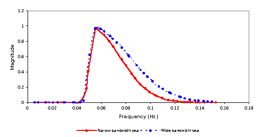 |
Figure 2
- Frequency components of typical narrow and wide bandwidth seas (40
components in range fl =0.05 -> fh=0.2 Hz)
Phase and Group Velocity: The sea surface
description used here is a travelling wave packet composed of a set
of Fourier components determined at one location which are then
individually phase shifted according to the requirements of the dispersion
relationship. This is the only manner in which the detailed shape of the
wave can be computed at a new location. Hence the propagation of
wave energy is not of explicit interest and so the phase velocity of
individual sinusoids that is of concern here not the group velocity.
4. Determination of maximum prediction time from a sea
spectrum
The
prediction techniques employed here1,2,3 are based upon using
sea surface measurements obtained at some distance from the prediction
site to estimate the coefficients in a dispersive wave-packet model of the
sea. This is essentially a spectral technique using the DFT to determine
the model coefficients. As the simulations are almost periodic functions
there is no natural periodic time to choose as a fundamental measurement
interval that will serve as the basic period for the Fourier Series
employed in building the sea-model. Consequently, unless corrective action
is taken, there will typically be strong windowing effects with each
spectral line in the prediction model (or in practice the actual sea
measurements) being substantially smeared by the window spectrum. This
effect can be dramatically reduced if the simulated (or measured) sea
surface waveforms are searched to find a new starting location whose value
and slope best match those of the most current data2,3. This
method makes the data sets used to determine the Fourier Series components
in the prediction model as nearly periodic as possible (thus minimising
windowing effects), while at the same time allowing the use of the
realistic non-periodic sea description to generate an ensemble of
simulations.
In
practice, this end matching is performed by first generating a data set of
some length, T seconds, substantially longer than is expected to be
required and then searching the oldest half of this waveform from its
start to find the best value and slope match to the most recent data
values. The start of the data set is then moved up to the best match point
resulting in a truncated waveform. The search region is restricted to the
first half of the data set in order to ensure an adequately long data
record.
The
truncated waveform is of varying length, and so the number of data samples
present is very unlikely to be equal to a power of two, consequently a
Fast Fourier Transform (FFT) cannot be employed directly to generate the
required spectra. The options are: to end pad the data with zeros; to
interpolate and resample the data using the optimal band limited
Sinc[xii]
based interpolation
polynomial or to use the Discrete Fourier Transform (DFT) directly. In
this case the DFT is employed.
For a
fixed measurement to prediction site distance, the prediction time
available is set by the velocities of the components at the high and low
frequency extremes of the sea spectrum. Thus, the wider the bandwidth of
the data used to build the prediction model, the shorter the possible
prediction time. As will be seen subsequently, the spectrum can be
significantly truncated thus increasing the possible prediction time
without introducing large errors.
Consequently, where possible, the simulated (or measured) sea surface
spectra should be truncated prior to constructing the space time diagram (Figure
1). Clearly, it is possible to continue
to truncate the sea spectrum to the point where operationally significant
components are being affected. This raises the important question of the
tradeoff between prediction time and prediction error, which will be
discussed later in the article.
Truncation is implemented by rejecting a percentage of the power spectrum
symmetrically at both its lower and upper ends although it can be argued
that there are some advantages in only removing the high frequencies. The
total spectral power rejection in the first set of results reported was
chosen to be 10% or less (5 % or less at each end of the spectrum). The
wavenumbers of the frequency components at the cut off points were
computed using the finite depth dispersion relationship (Equation 3).
Equation 3
where h
is the sea depth, g is the local gravitational constant, k is the
wavenumber and
w
= 2pf
is the angular frequency. The geometry of the space time diagram (Figure
1) is then used to determine the maximum
prediction time possible.
5. Variation of maximum
prediction time and optimal distance with sea depth and measurement time
window
Figure 3 illustrates the effects on maximum
prediction time of increasing sea depth. This is shown for measurement
time windows of 32 s, 64 s and 128 s. The effects on optimal distance of
increasing sea depth are shown in Figure 4. Points plotted in Figure 3 and
Figure 4 are the results of an average of 100 random sea waveforms
produced using the model sea spectrum shown in Figure 2. The standard
deviations of the populations for each point are also shown.
It is apparent from Figure 3 that maximum
prediction time diminishes with increasing sea depth which is in accord
with the general trend toward an increase in wave velocity for all
frequency components leading to steeper line slopes on the space time
diagram.
Figure 3
also illustrates as expected2,3, that the maximum prediction
time and the distance at which this occurs increase proportionately with
the measurement time window. Specifically, the maximum prediction time for
deep water where phase velocity varies inversely with frequency is given
by:
Tmax
= T fl / fh
(4)
i.e., independent of water depth. However
in shallower waters where the general form of equation 3 must be used the
results become depth dependent. The form of 3 suggests the expected trend
is for prediction time to decrease with increasing depth asymptotically
toward the deep water behaviour and this is born out in the simulations.
The converse is expected for the optimum distance and again this is
observed to be the case.
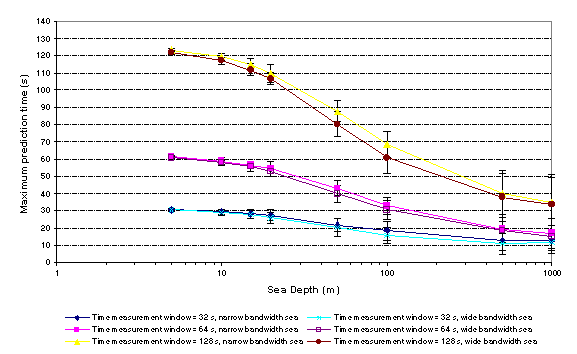
Figure 3 – The
variation of maximum prediction time with increasing sea depth for
measurement time windows of 32 s, 64 s and 128 s. The standard deviations
of each point are also shown (population size = 100).
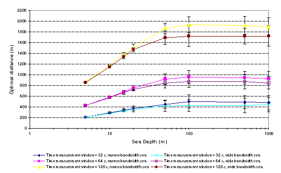
Figure
4 - The
variation of optimal distance with increasing sea depth for measurement
time windows of 32 s, 64 s and 128 s. The standard deviations of each
point are also shown (population size = 100).
The effects on maximum prediction time and
optimal distance of varying the set spectral power rejection percentage
for measurement time windows of 32s, 64 s and 128 s and sea depths of 20 m
and 500 m are illustrated in Figure 5 and Figure 6. The points plotted in
Figure 5 and Figure 6 are the results of an average of 100 random sea
waveforms produced from the sea model spectrum shown in Figure 2. The
standard deviations of the populations for each point are also shown. The
sensitivity of the deep water prediction times estimates to the sea
bandwidth is evident in equation 4 for the case of maximum prediction time
and are equally evident from figure 1 for more general
conditions as well. The gains achieved by truncating the spectra used for
prediction estimates are evident in figure 5 together with the associated
changes in the distance required for optimal prediction time. Clearly such
truncation corresponds to rejecting input data and hence the horizontal
axis in figure 5 is related to the level of error introduced
by truncation. An important feature of the results is that after an
initial rapid rise the incremental error introduced becomes modest and is
to be expected because the ratio fl/fh
Þ 1.
An
additional important factor is the effect of the bandwidth upon the
computational time required by the prediction algorithms. This issue is
examined subsequently in Section 8.
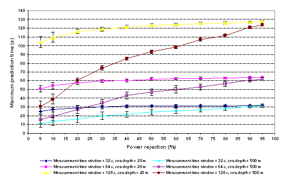
Figure 5 - Variation of maximum prediction time with set spectral power
rejection, measurement time window and sea depth for a narrow bandwidth
sea. Standard deviations are shown for each point.
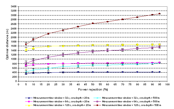
Figure 6 - - Variation of optimal distance with set
spectral power rejection, measurement time window and sea depth for a
narrow bandwidth sea. Standard deviations are shown for each point.
As expected from the space time diagram,
prediction times increase with spectral truncation, and consequently with
prediction error. This reflects the fact that the difference in velocity
between the limiting components reduces and the lines forming the
prediction triangle (Figure 1) become increasingly parallel.
7. Variation of prediction time with the distance between measurement and
prediction site and measurement time window
Figure 7 shows the relationship between
prediction time and separation between measurement and prediction sites
for shallow and deep water. The main difference between the results for
shallow and deep water is the more moderate fall off of prediction time
with distance in the shallow water case. This reflects the fact that in
the limit as kh ® 0 the phase
velocity is constant and the sides of prediction triangle (Figure 1)
become more parallel. For deep water the lines representing fl
and fh in Figure 1 become more steep, thereby reducing the
maximum prediction time possible.
|
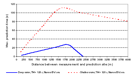 |
Figure 7 – Illustration of the variation of
prediction time with the distance between measurement and prediction site
for shallow and deep water (using the 40 component wide bandwidth sea
model with sea depth = 20 m and sea depth = 500 m).
8. Practical Applications
In the application of DSWP to a marine
problem, the most likely specifications will involve the minimum useful
prediction time and/or the fraction of the time which predictions can be
made for. In designing a DSWP system to meet such specifications there
will be essentially three classes of parameter. Firstly there are factors
such as the depth of water and the current sea state which are outside the
operator’s control. Secondly there will be basic system parameters that
will mainly be set at the design stage, e.g., in the Fixed Point method
under discussion here, an example might be the separation of the
measurement and prediction points. The remaining parameters such as the
measurement time duration, type of end matching used and the degree of
spectral truncation are under operator control and may be varied to
achieve the specification for the prevailing sea conditions. Examples of
possible applications in the offshore oil industry include direct ship to
rig personnel transfers and craning of materials to and from supply
vessels.
An example system
As an example of the type of issues that
must be examined when designing a DSWP system consider the factors
affecting a steerable gangway of the type being proposed for personnel
transfers between oil rigs and service vessels. Wave prediction is needed
for two reasons. Firstly to make a safe initial connection of the gangway
to the vessel and secondly to warn of impending dangerous relative motion
between ship and rig. Assume for the sake of illustration that 20 seconds
would be a minimum acceptable prediction time to be useful. Next the
acceptable error tolerance in predicting the vessel motion must be
defined. This serves to define the acceptable prediction error.
Consequently it sets the limits on the combination of the best possible
performance required of the basic DSWP system together with allowances for
any de-rating of this precision due to spectral truncation. This may be
needed to provide the capability for extension of prediction times, albeit
at reduced precision, beyond those achievable with the basic DSWP system
under the prevailing conditions.
In order to address the required
specification it is first necessary to consider the worst case sea type
that the system will be used for. In practice this is likely to involve a
set of simulation studies, however for simplicity it is assumed here that
the wide bandwidth version of the 40 component non-uniform spectrum
employed previously provides a satisfactory description of these
conditions. Clearly as linear analysis is used there is no requirement to
specify the actual wave amplitude scale.
Important compromises may be identified
when establishing the optimum distance for the wave sensors (measurement
site) from the rig (prediction site). If this distance is too short, then
the maximum possible prediction time is limited. If the distance is too
long then prediction errors due to second order non-linear processes8,
and errors in the knowledge of the wave direction and sea spectrum become
significant. Wind induced waves generated between the measurement and
prediction sites are unlikely to be significant over the typical distances
used. To obtain the best performance from the system, therefore, the aim
is to place the wave measuring sensors as close to the rig as possible,
compatible with meeting the required prediction time specification under
the given or expected conditions. Figure 7 provides data for two cases, 20
m and 500 m depth, where the sensor distances are 250m and 1300m
respectively. It is useful to recall that the maximum prediction time for
a given distance corresponds to the propagation time from the measurement
to the prediction site of the slowest wave component considered. In the
present case the slowest wave velocities are 11.7 ms-1 for 20 m depth and
14.6 ms-1 for 500 m depth giving corresponding measurement
times of 23.0 s and 90.0 s. However this does not allow for the end
matching processes needed to minimise the departure from periodicity in
the data. If the present approach is used, whereby up to 50% of the data
record may be rejected, the measurement times must be twice the above
values.
Since wave data would almost certainly be
logged continuously the measurements would be implemented on a moving
window basis. The shortest time between predictions would be set by the
computational demands of model building as outlined in the following
section.
Computational effects upon prediction time.
In addition to the
analytical factors affecting the choice of measurement times it must be
recognised that there are significant computational overheads. The net
prediction time available is the balance left after all computational
costs have been deducted from the theoretical prediction time as described
so far. This mainly arises because of the need to wait until all the data
is collected before performing the end matching process.
There are a variety
of options available for carrying out the spectral estimates required
for prediction determinations. To some extent these depend upon
whether a Fast Fourier Transform algorithm,(FFT), or a direct evaluation
of the inner product, (DFT), is employed. As will be demonstrated the
choice of approach does not simply depend upon the lower execution time
for the FFT. The various possibilities will be discussed below and as
might be anticipated a compromise has to be made between precision and the
net prediction time $T_{net}$ available after computational overheads.
When using a DFT the
maximum possible value of $T_{net}$ tends for a large number of data
points, $N$, to the value:
$$
T_{net,DFT} = {1\over{t_{mlt}}}{f_{min}\over{(2f_{max})^2}}\eqno(4)
$$
where $f_{min}$ and $f_{max}$
are respectively the minimum and maximum frequencies used
and $y_{mlt}$ is the execution time for floating point
multiplication.
The equivalent result
for an FFT algorithm is:
$$
T_{net,FFT} = {2\>t_{mlt}\>log_e2\over{2^{log_e2}}}\>
2^{ \Bigl\lbrace{f_{min}\over{ (2f_{max})^2 \>t_{mlt} }} \Bigr\rbrace
}\eqno(5)
$$
hence speed up ratio
of FFT to DFT si given by:
$$
{T_{net,FFT}\over{T_{net,DFT}}} = {2\>log_e2\over{2^{log_e2}
}}\>\>\>{2^\beta \over{\beta^2}}
\eqno(6)
$$
where
$$
\beta \qquad = \qquad {f_{min}\over{(2 \>f_{max})^2\>t_{mlt}}}\eqno(7)
$$
\vfill\eject
For the typical
values quoted previously $\beta \gg 1$ and so as expected the gains
in using an FFT over a DFT appear to be very large. However there
are additional computational costs associated with the requirement of the
FFT to have $2^M$ points, with $M$ an integer. To achieve this the
original $N$ point data set requires re-sampling
using some form of interpolation algorithm to produce $2^M$ new values
where both $M$ and the new sample interval $\delta t_2$ must be
chosen to satisfy:
$$
2^M\> \delta t_2 \qquad = \qquad T
$$
where as previously
$T$ is the duration of the end matched data set. Clearly the new sampling
rate ${1\over{\delta t_2}}$ must also satisfy the sampling requirement.
The additional computational cost is associated with the interpolation
process. Given that the data is band limited to
$\>\omega_c\> \geq \>{\pi\over{f_{max}}}\>$ it is possible to use the
reconstruction polynomial associated with Nyquist’s Sampling Theorem that
in principle allows an exact reconstruction of band limited data. The
resulting new sample set, $f_R[k]$ is then given by:
$$
f_R[k] \qquad = \qquad \sum^\infty_{\ell=-\infty} f\Bigl(\ell \>{T\over{N}}\Bigr)
{ sin\Bigl\{\omega_c(k{T\over{2^M}} - \pi\ell)\Bigr\} \over{\omega_c(k{T\over{2^M}}
- \pi\ell)}}\eqno(9)
$$
where the $f\Bigl(\ell
\>{T\over{N}}\Bigr)$ are the original data set. Clearly the actual data
set is finite thus equation (9) is a finite sum over $N$, not infinte sum.
Furthermore even a full finite evaluation would require $N^2$
multiplications which is the same order as the DFT and would thus
completely remove any advantage in using the FFT algorithm. Consequently
the summation must be truncated, thus compromising accuracy to some
extent. This leaves only a modest number of points, designated $2R$, local
to $k$ which actually contribute to $f_R[k]$ and equation (9) becomes:
$$
f_R[k] \qquad = \qquad \sum^{k + R}_{\ell= k - R} f\Bigl(\ell \>{T\over{N}}\Bigr)
{ sin\Bigl\{\omega_c(k{T\over{2^M}} - \pi\ell)\Bigr\} \over{\omega_c(k{T\over{2^M}}
- \pi\ell)}}\eqno(10)
$$
Even the truncated
interpolation function requires an execution time of $2\>R\>2^M \delta (t_{mlt}+t_{sinc})$
where $t_{sinc}$ is the evalution time for the $sinc$
function which can easily exceed the demands of the FFT itself and also
introduces additional approximation. This is the reason for the
earlier statement that the choice between the
use of an FFT or a DFT is not so clear cut as the simple spectral
computation time ratio in equation (6) might suggest.
An alternative
approach is to dispense with the end matching process and accept the
consequent level of error$^{2a}$. This makes it possible to adopt a
predefined fixed number of sample points and
allows the DFT inner product sums for each harmonic to be evaluated
cumulatively as the data values arrive. Given the typical sampling times
and the fact that the measurement interval must always exceed the
prediction time then to all practical purposes DFT based spectral
calculations can be completed by the end of the measurement interval. Thus
there is no detraction from the prediction time. This cannot be achieved
with the FFT as all the data points are needed at the outset.
Practical Conclusion
Concerning Computational Costs
The above discussion
explains the statement made at the beginning of this section, i.e., that
there are a substantial number different ways of handling the affect of
computational load on total prediction time. Hardly surprisingly these
involve a range
of choices between
prediction time and precision. Whichever option or combination of
options is adopted
depends very much upon the applications goal. If the most important thing
is to have some predictive estimates available at all times even if they
have modest precision, then a sensible route is to use a fixed number of
samples and employ the cumulative DFT based evaluation scheme. If higher
accuracy is needed but prediction estimates are acceptable for less of the
time then a combination of end matching and an FFT using a moderate length
interpolation function is a reasonable choice. If the extra procession
cost is tolerable a better overal approach would be to run both
methodologies in parallel.
It is important to
stress that it is essential to also monitor the more traditional power
spectral information as this determines the average properties of
the sea which are required in order to make initial bound estimates of key
parameters such as the upper and lower frequencies to be used and hence to
likely range of measurement times required. Such data can obviously be
derived by accumulating the basic wave data.
The more realistic
multi-directional situation also involves decomposing a sea into a set of
R dominant one dimensional long crested swells then making spectral
estimates associated with the R independent data sets required. The
directions of these swells together with their associated magnitudes and
phases, which are all needed for prediction, are then determined by
solving a system of R spectral equations. As R is typically modest,
typically 3 to 6 depending upon conditions the main additional cost is
thus the R fold increase in the time for making spectral estimates.
Acknowledgements
The authors would
like to thank DERA Bedford for helping support this work and to Dr.K.Wadee
for helpful suggestions on certain numerical analysis issues.
  |
